Conditional RNN in keras (R) to deal with static features

Mar 5, 2022 r keras

Conditional RNN is one of the possible solutions if we’d like to make use of static features in time series forecasting. For example, we want to build a model, which can handle multiple time series with many different characteristics. It can be a model for demand forecasting for multiple products or a unified model forecasting temperature in places from different climate zones.

We have at least a couple of options to do so. They are described in detail in the following thread on StackOverlow. According to the answers, the best way to add static features is to use this values to produce an initial hidden state of the recurrent layer. The proposed solution was implemented as a Keras wrapper to recurrent layers (in Python).

This post is a trial to implement conditional RNN in keras for R.

Loading the data

We’ll use a piece of data from an experiment performed by the author of the aforementioned Keras wrapper. We’re selecting two cities with extreme temperatures, e.g. Cairo and Helsinki.

library(data.table, warn.conflicts = FALSE)
library(dplyr, warn.conflicts = FALSE)
library(lubridate)
library(ggplot2)
library(imputeTS
library(timetk)
library(rsample)
library(parsnip)

# url       <- "https://github.com/philipperemy/cond_rnn/raw/master/examples/temperature/city_temperature.csv.zip"
file_path <- "city_temperature.csv.zip"
csv_path  <- "city_temperature.csv"

# download.file(url, file_path)
# unzip(file_path)

city_temperature <- read.csv(csv_path)
setDT(city_temperature)

selected_cities <- 
  city_temperature[City %chin% c('Cairo', 'Helsinki')]

selected_cities[
  , Date := ymd(glue::glue("{Year}-{Month}-{Day}", .envir = .SD))
]

selected_cities <- 
  selected_cities[, .(City, Date, AvgTemperature)]
setorder(selected_cities, City, Date)

plt <- 
  ggplot(selected_cities) +
  geom_line(aes(Date, AvgTemperature, col = City)) + 
  theme_minimal() +
  ggtitle("Temperature: Cairo vs Helsinki")

plt

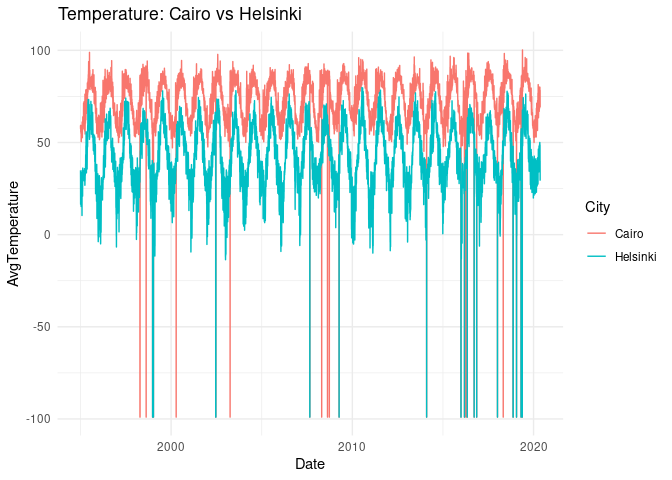
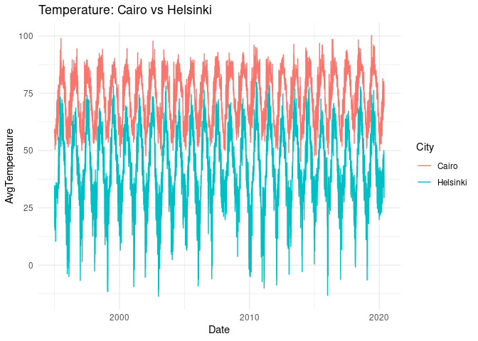
There is a couple of outliers and we can safely assume they simply indicate lack of data. We’ll replace it with interpolated values.

Initially, I’ve chosen Oslo, but there were a few corrupted year numbers:

city_temperature[City == 'Oslo' & Year == 200]

##     Region Country State City Month Day Year AvgTemperature
##  1: Europe  Norway       Oslo    12   1  200            -99
##  2: Europe  Norway       Oslo    12   2  200            -99
##  3: Europe  Norway       Oslo    12   3  200            -99
##  4: Europe  Norway       Oslo    12   4  200            -99
##  5: Europe  Norway       Oslo    12   5  200            -99
##  6: Europe  Norway       Oslo    12   6  200            -99
##  7: Europe  Norway       Oslo    12   7  200            -99
##  8: Europe  Norway       Oslo    12   8  200            -99
##  9: Europe  Norway       Oslo    12   9  200            -99
## 10: Europe  Norway       Oslo    12  10  200            -99
## 11: Europe  Norway       Oslo    12  11  200            -99
## 12: Europe  Norway       Oslo    12  12  200            -99
## 13: Europe  Norway       Oslo    12  13  200            -99
## 14: Europe  Norway       Oslo    12  14  200            -99
## 15: Europe  Norway       Oslo    12  15  200            -99
## 16: Europe  Norway       Oslo    12  16  200            -99
## 17: Europe  Norway       Oslo    12  17  200            -99
## 18: Europe  Norway       Oslo    12  18  200            -99
## 19: Europe  Norway       Oslo    12  19  200            -99
## 20: Europe  Norway       Oslo    12  20  200            -99
## 21: Europe  Norway       Oslo    12  21  200            -99
## 22: Europe  Norway       Oslo    12  22  200            -99
## 23: Europe  Norway       Oslo    12  23  200            -99
## 24: Europe  Norway       Oslo    12  24  200            -99
## 25: Europe  Norway       Oslo    12  25  200            -99
## 26: Europe  Norway       Oslo    12  26  200            -99
## 27: Europe  Norway       Oslo    12  27  200            -99
## 28: Europe  Norway       Oslo    12  28  200            -99
## 29: Europe  Norway       Oslo    12  29  200            -99
## 30: Europe  Norway       Oslo    12  30  200            -99
## 31: Europe  Norway       Oslo    12  31  200            -99
##     Region Country State City Month Day Year AvgTemperature

# Cleaning the data
selected_cities[AvgTemperature == -99.0, AvgTemperature := NA]
selected_cities[, AvgTemperature := na_interpolation(AvgTemperature)]

plt <- 
  ggplot(selected_cities) +
  geom_line(aes(Date, AvgTemperature, col = City)) + 
  theme_minimal() +
  ggtitle("Temperature: Cairo vs Helsinki")

plt
# plotly::ggplotly(plt)

library(tsibble, warn.conflicts = FALSE, quietly = TRUE)

duplicates(selected_cities, key = City, index = Date)

## # A tibble: 4 × 3
##   City     Date       AvgTemperature
##   <chr>    <date>              <dbl>
## 1 Cairo    2015-12-30           60.5
## 2 Cairo    2015-12-30           57.9
## 3 Helsinki 2015-12-30           26.6
## 4 Helsinki 2015-12-30           25.4

# Removing dupicates for 
selected_cities <- 
  selected_cities[, .(AvgTemperature = max(AvgTemperature)) , by = .(City, Date)]

train <- selected_cities[Date < as.Date('2019-01-01')]
test  <- selected_cities[
  Date >= as.Date('2019-01-01') & Date <= as.Date('2019-12-31')
]

Baseline model - one xgboost model for both cities

As a baseline model, we’ll train a xgboost model using parsnip API and modeltime. We create a data.frame of lagged variables to feed the model. We use 28 lags - the same value will be later used as a length of input to the recurrent neural netowrk models. We also mix the data belonging to different cities, so there are no separate models for each city.

library(modeltime)

lagged_selected_cities <- 
  selected_cities %>% 
  group_by(City) %>% 
  tk_augment_lags(AvgTemperature, .lags = 1:28) %>% 
  ungroup()

setDT(lagged_selected_cities)

train <- lagged_selected_cities[Date < as.Date('2019-01-01')]
test  <- lagged_selected_cities[
  Date >= as.Date('2019-01-01') & Date <= as.Date('2019-12-31')
]

lagged_variables <- glue::glue("AvgTemperature_lag{1:28}")
formula_rhs      <- paste0(lagged_variables, collapse = " + ")
model_formula    <- as.formula(
  glue::glue("AvgTemperature ~ {formula_rhs}")
)

model_xgboost <- 
  boost_tree(mode = "regression") %>% 
  set_engine("xgboost") %>% 
  fit(model_formula, data = train)

fcast <- 
  model_xgboost %>% 
  predict(test)

mdltime <- 
  modeltime_table(
    xgboost = model_xgboost
  )

fcast_cairo <- 
  mdltime %>% 
  modeltime_forecast(
    test[City == 'Cairo'], actual_data = test[City == 'Cairo']
  ) 

fcast_helsinki <- 
  mdltime %>% 
  modeltime_forecast(
    test[City == 'Helsinki'], actual_data = test[City == 'Helsinki']
  ) 

fcast_cairo <- 
  fcast_cairo %>% 
  mutate(name = 'Cairo')

fcast_helsinki <- 
  fcast_helsinki %>% 
  mutate(name = 'Helsinki')

fcast_xgboost <- 
  bind_rows(
    fcast_cairo, fcast_helsinki
  ) %>% 
  filter(.key == 'prediction') %>% 
  select(.index, .value, name) %>% 
  rename(Date = .index, value = .value) %>% 
  mutate(model = 'xgboost')

Let’s take a glance, how the models’ predictions look like.

fcast_xgboost_cmp <- 
  bind_rows(
    fcast_xgboost,
    select(test, Date, name = City, value = AvgTemperature) %>% 
      mutate(model = 'actual')
  )

ggplot(fcast_xgboost_cmp) + 
  geom_line(aes(Date, value, col = model)) + 
  facet_wrap(~name) +
  theme_minimal()

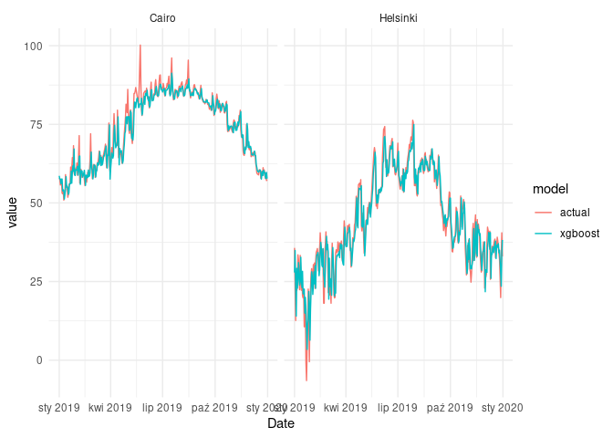
As we can see, xgboost models fitted to the data quite well. However, the task was relatively simple, because we only wanted to forecast one timestep ahead.

Preparing data for RNNs

We pass to the ‘main course’ - training recurrent neural networks. First, we create a couple of auxiliary functions to create input tensors:

3-dimensional tensors for input time series
matrices for outputs and static variables

library(abind)

ndim <- function(x){
  length(dim(x))
}

shuffle <- function(...){

  objects     <- list(...)
  object_size <- dim(objects[[1]])[1]
  
  indices <- sample(object_size,  object_size)
  
  Map(\(x) if (ndim(x) == 2) x[indices, ] else x[indices, ,], objects)
}

prepare_output <- function(fcast, idx){

  idx_cairo    <- idx == 1
  idx_helsinki <- idx == 0
    
  fcast_cairo <- 
    fcast[idx_cairo, ] %>% 
    t() %>% 
    as.vector()
  
  fcast_helsinki <- 
    fcast[idx_helsinki, ] %>% 
    t() %>% 
    as.vector()
  
  fcast_df <- 
    data.table(
      Date = test$Date[1:length(fcast_cairo)],
      Cairo = fcast_cairo,
      Helsinki = fcast_helsinki
    ) %>% 
    tidyr::pivot_longer(c(Cairo, Helsinki))
  
    fcast_df
}

prepare_data <- function(data, timesteps, horizon, jump, 
                       sample_frac, targets = TRUE, .shuffle = TRUE){

  data_period_length <- max(data$Date) - min(data$Date)
  data_period_length <- as.numeric(data_period_length) + 1
  
  n <- data_period_length - timesteps - horizon + 1
  
  starts <- seq(1, n, jump)
  starts <- sample(starts, size = length(starts) * sample_frac)
  starts <- sort(starts)
  
  # Cairo
  data_cairo <- 
    data[City == 'Cairo', .(AvgTemperature)]
  
  x_data_cairo <- 
    purrr::map(
      starts, 
      \(i) array(data_cairo[i:i+timesteps-1, ]$AvgTemperature, c(1, timesteps, 1))
    )
  
  x_data_cairo        <- abind(x_data_cairo, along = 1)
  x_data_static_cairo <- matrix(1, dim(x_data_cairo)[1], 1) 
  
  y_data_cairo <- 
      purrr::map(
        starts, 
        \(i) array(data_cairo[(i+timesteps):(i+timesteps+horizon-1), ]$AvgTemperature, c(1, horizon))
      )
  y_data_cairo <- abind(y_data_cairo, along = 1)
  
  # Helsinki
  data_helsinki <- 
    data[City == 'Helsinki', .(AvgTemperature)]
  
  x_data_helsinki <- 
    purrr::map(
      starts, 
      \(i) array(data_helsinki[i:i+timesteps-1, ]$AvgTemperature, c(1, timesteps, 1))
    )
  
  x_data_helsinki        <- abind(x_data_helsinki, along = 1)
  x_data_static_helsinki <- matrix(0, dim(x_data_helsinki)[1], 1) 
  
  # Complete data
  x_data        <- abind(x_data_cairo, x_data_helsinki, along = 1)
  x_static_data <- abind(x_data_static_cairo, x_data_static_helsinki, along = 1) 
  
  right_order <- 
  
  if (targets) {
      y_data_helsinki <- 
      purrr::map(
        starts, 
        \(i) array(data_helsinki[(i+timesteps):(i+timesteps+horizon-1), ]$AvgTemperature, c(1, horizon))
      )
      
      y_data_helsinki <- abind(y_data_helsinki, along = 1)
      y               <- abind(y_data_cairo, y_data_helsinki, along = 1)
      
      if (.shuffle)
        return(shuffle(x_data, x_static_data, y))
      else
        return(list(x_data, x_static_data, y))
  } else {
    if (.shuffle)
      return(shuffle(x_data, x_static_data))
    else 
      return(list(x_data, x_static_data))
  }

}

Experiment configuration:

TIMESTEPS        <- 28
HORIZON_1        <- 1
HORIZON_7        <- 7

DYNAMIC_FEATURES <- 1
STATIC_FEATURES  <- 1
RNN_UNITS        <- 32
VOCABULARY_SIZE  <- 2 # because we have two cities

Importing keras, we’re also loading multiple assignment operator from zeallot, namely %<-%.

library(keras)

JUMP        <- 1
SAMPLE_FRAC <- 0.5

# HORIZON = 1

# Training data
c(x_train_h1, x_static_train_h1, y_h1) %<-% 
  prepare_data(
    data        = train,
    timesteps   = TIMESTEPS,
    horizon     = HORIZON_1,
    jump        = HORIZON_1,
    sample_frac = SAMPLE_FRAC
  )

# Test data
c(x_test_h1, x_static_test_h1) %<-% 
  prepare_data(
    data        = test,
    timesteps   = TIMESTEPS,
    horizon     = HORIZON_1,
    jump        = HORIZON_1,
    sample_frac = 1,
    targets     = FALSE,
    .shuffle    = FALSE 
  )

# HORIZON = 7

# Training data
c(x_train_h7, x_static_train_h7, y_h7) %<-% 
  prepare_data(
    data        = train,
    timesteps   = TIMESTEPS,
    horizon     = HORIZON_7,
    jump        = 1,
    sample_frac = SAMPLE_FRAC
  )

# Test data
c(x_test_h7, x_static_test_h7) %<-% 
  prepare_data(
    data        = test,
    timesteps   = TIMESTEPS,
    horizon     = HORIZON_7,
    jump        = HORIZON_7,
    sample_frac = 1,
    targets     = FALSE,
    .shuffle    = FALSE 
  )

Conditional RNN

The idea of conditional RNN is to initialize hidden states of the recurrent layer using specially prepared values, which indicate a specific type of the time series.

I let myself for some simplifications in these experiments, e.g.:

data is not scaled
validation data is not used to prevent overfitting

experiment_conditional_rnn <- 
    function(timesteps, horizon, rnn_units, 
            vocabulary_size, dynamic_features, static_features,
            model, x_train, x_static_train, y, x_test, x_static_test){

  # Model
  ts_input     <- layer_input(shape = c(timesteps, dynamic_features))
  static_input <- layer_input(shape = static_features)
  
  embedding <- layer_embedding(input_dim = vocabulary_size, 
                               output_dim = rnn_units)(static_input)
  embedding <- layer_lambda(f = \(x) x[,1,])(embedding)
  
  rnn_layer <- 
    layer_gru(units = rnn_units, name = 'rnn')(ts_input, initial_state = embedding)
  
  # For LSTM layers we have to provide two hidden state values
  # rnn_layer <- 
  #  layer_gru(units = rnn_units, name = 'rnn')(ts_input, initial_state = list(embedding, embedding))
  
  final_layer <- layer_dense(units = horizon, activation = 'linear')(rnn_layer)
  
  # Compiling
  net <- 
    keras_model(
      inputs  = list(ts_input, static_input),
      outputs = list(final_layer) 
    ) %>%
    compile(
      optimizer = 'adam',
      loss      = 'mae'
    )
  
  # Training
  net %>% 
    fit(
      x = list(x_train, x_static_train),
      y = list(y),
      epochs = 50,
      batch_size = 32
    )

  # Forecasting
  fcast <- 
    net %>% 
    predict(list(x_test, x_static_test))
  

  fcast_df <- prepare_output(fcast, x_static_test)
  fcast_df$model <- model

  list(net, fcast_df)
}

# HORIZON = 1
c(net_cond_h1, fcast_cond_h1) %<-% 
  experiment_conditional_rnn(
    # Network
    timesteps        = TIMESTEPS,
    vocabulary_size  = VOCABULARY_SIZE,
    dynamic_features = DYNAMIC_FEATURES,
    static_features  = STATIC_FEATURES,
    horizon          = HORIZON_1,
    rnn_units        = RNN_UNITS,
    model            = 'cond_rnn_h1',
    # Data
    x_train          = x_train_h1,
    x_static_train   = x_static_train_h1,
    y                = y_h1,
    x_test           = x_test_h1,
    x_static_test    = x_static_test_h1
  )

## Loaded Tensorflow version 2.8.0

# HORIZON = 7
c(net_cond_h7, fcast_cond_h7) %<-% 
  experiment_conditional_rnn(
    # Network
    timesteps        = TIMESTEPS,
    vocabulary_size  = VOCABULARY_SIZE,
    dynamic_features = DYNAMIC_FEATURES,
    static_features  = STATIC_FEATURES,
    horizon          = HORIZON_7,
    rnn_units        = RNN_UNITS,
    model            = 'cond_rnn_h7',
    # Data
    x_train          = x_train_h7,
    x_static_train   = x_static_train_h7,
    y                = y_h7,
    x_test           = x_test_h7,
    x_static_test    = x_static_test_h7
  )

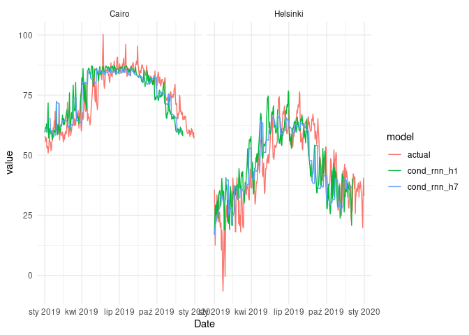
fcast_cond_cmp <- 
  bind_rows(
    fcast_cond_h1,
    fcast_cond_h7,
    select(test, Date, name = City, value = AvgTemperature) %>% 
      mutate(model = 'actual')
  )

ggplot(fcast_cond_cmp) + 
  geom_line(aes(Date, value, col = model)) + 
  facet_wrap(~name) +
  theme_minimal()

Simple RNN

experiment_simple_rnn <- 
  function(timesteps, horizon, rnn_units,
           model, x_train, y, x_test, x_static_test){
  
  # Network architecture
  ts_input  <- layer_input(shape = c(timesteps, 1))
  rnn_layer <- layer_gru(units = rnn_units, name = 'rnn')(ts_input)
  
  final_layer <- 
    layer_dense(units = horizon, activation = 'linear')(rnn_layer)
  
  # Compiling
  net <- 
    keras_model(
      inputs  = list(ts_input),
      outputs = list(final_layer) 
    ) %>%
    compile(
      optimizer = 'adam',
      loss      = 'mae'
    )
  
  # Training 
  net %>% 
    fit(
      x = list(x_train),
      y = list(y),
      epochs = 50,
      batch_size = 32
    )
  
  # Forecasting
  fcast <- 
    net %>% 
    predict(list(x_test))
  
  fcast_df <- prepare_output(fcast, x_static_test)
  fcast_df$model <- model

  list(net, fcast_df)     
}

# HORIZON = 1
c(net_simple_h1, fcast_simple_h1) %<-% 
  experiment_simple_rnn(
    # Network
    timesteps     = TIMESTEPS,
    horizon       = HORIZON_1,
    rnn_units     = 32,
    model         = 'simple_rnn_h1',
    # Data
    x_train       = x_train_h1,
    y             = y_h1,
    x_test        = x_test_h1,
    x_static_test = x_static_test_h1
  )

# HORIZON = 7
c(net_simple_h7, fcast_simple_h7) %<-% 
  experiment_simple_rnn(
    # Network
    timesteps     = TIMESTEPS,
    horizon       = HORIZON_7,
    rnn_units     = 32,
    model         = 'simple_rnn_h7',
    # Data
    x_train       = x_train_h7,
    y             = y_h7,
    x_test        = x_test_h7,
    x_static_test = x_static_test_h7
  )

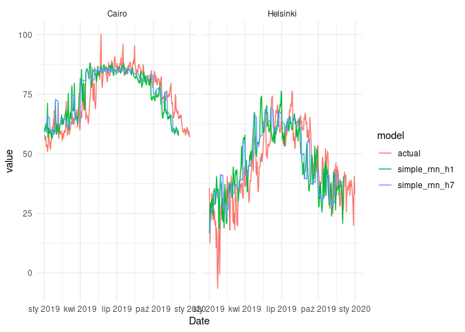
fcast_simple_cmp <- 
  bind_rows(
    fcast_simple_h1,
    fcast_simple_h7,
    select(test, Date, name = City, value = AvgTemperature) %>% 
      mutate(model = 'actual')
  )

ggplot(fcast_simple_cmp) + 
  geom_line(aes(Date, value, col = model)) + 
  facet_wrap(~name) +
  theme_minimal()

Summary

library(yardstick)

fcast_df <- 
  bind_rows(
    fcast_xgboost,
    fcast_cond_h1,
    fcast_cond_h7,
    fcast_simple_h1,
    fcast_simple_h7
  )

fcast_df <- 
  fcast_df %>% 
  left_join(test %>% select(Date, City, AvgTemperature), 
            by = c('Date', 'name'='City'))

fcast_df %>% 
  group_by(model) %>% 
  summarise(mape = mape_vec(AvgTemperature, value)) %>% 
  gt::gt()

model	mape
cond_rnn_h1	34.32918
cond_rnn_h7	31.92488
simple_rnn_h1	34.44923
simple_rnn_h7	32.86985
xgboost	14.82363

plt <- 
  ggplot(fcast_df) + 
  geom_line(aes(Date, value, col = model)) + 
  theme_minimal() +
  facet_wrap(~name)

plt

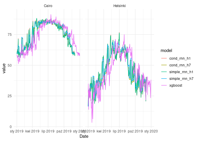
Conclusions

As we can see, there is technically no difference in terms of MAPE, when we are comparing results of simple_rnn_h1 and cond_rnn_h1. When it comes to the RNN models with 7-day horizon, the diffrences are also negligible.

Our baseline model beats both simple and conditional RNN models. However, bear in mind that 1-timestep horizon is not a most realistic use case in most problems.