How icy is sun, how fiery is snow? Playing with word embedding vectors
en python word embedding nlp mathWe all know old, good and hackneyed examples, that are typically used to intuitively explain, what the word embedding technique is. We almost always come across a chart presenting a simplified, 2-dimensional vector representation of the words queen and king, which are distant from each other similarly as the words woman and man.
Today, I’d like to go one step further and explore the meaning of the mutual position of two arbitrary selected vectors. It this particular case - relation between the ice-and-fire pair and the rest of the vectors.
Motivation
Assume for the moment we have an embedding in the 2-dimensional space. It’s not a realistic case, because normally such low-dimensional embedding wouldn’t fulfill its purpose. So, we have a bunch of vectors or points, described with two coordinates. We choose two such vectors, say ice and fire, as mentioned above.
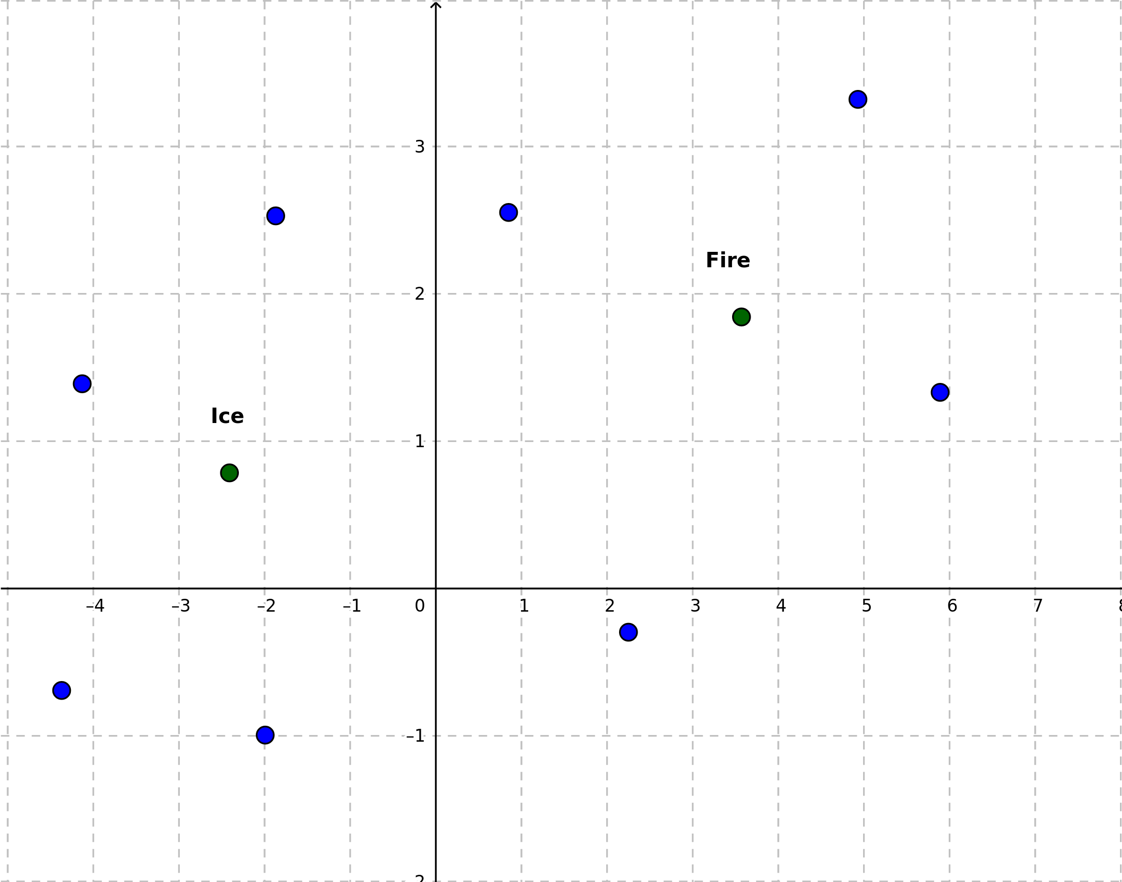
Treating the straight line passing trough these points as a new axis, we project the rest of the points onto this line. The midpoint between “ice” and “fire” can be treated as the origin (“point 0”) of the new axis.
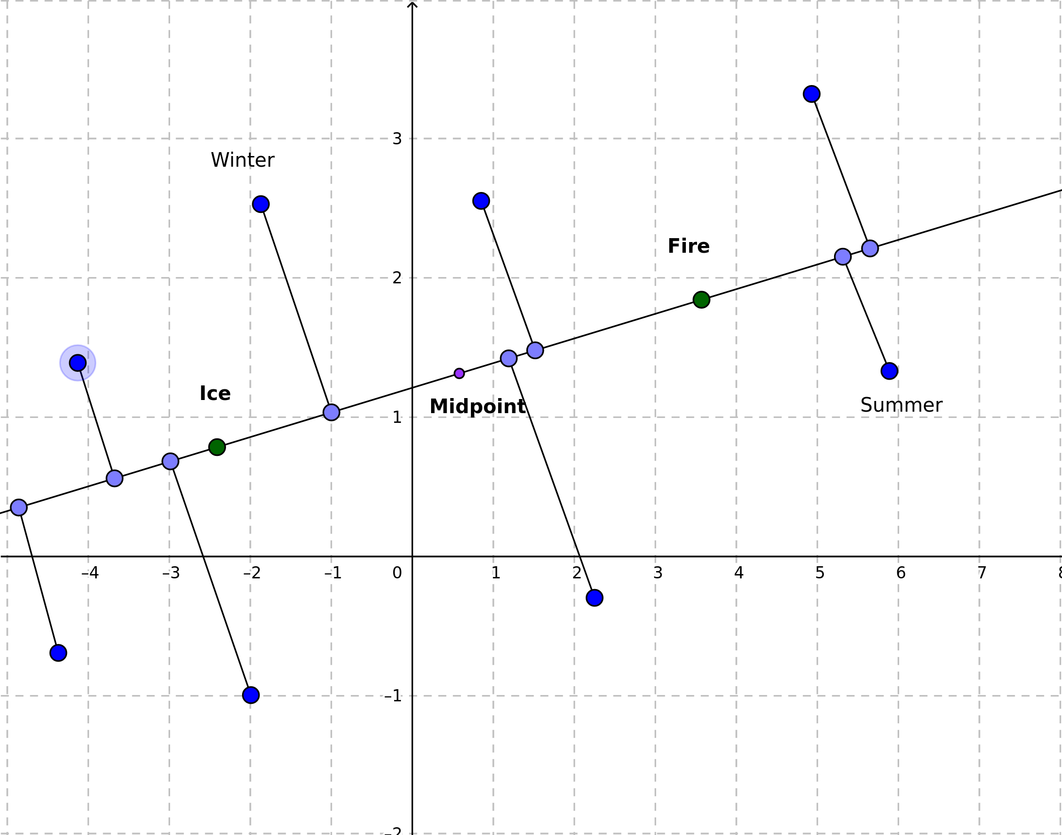
I will call the ice and fire points poles, to express that they show us, what is the expected meaning of being “negative” and “positive”. Briefly - I expect that embedding vectors (poinst) for “cold” words such as “winter” will get a negative value on this new axis, while “warm” words - positive values. In this context it means that positive-valued points are those ones, that have their projections on the “right” side of the of the new axis.
Values obtained for each point are the distances from the projections to the midpoint (with sign).
Math & code behind
One of the most convenient ways to get embedding vectors for natural language is to use pre-trained models distributed with spacy library.
import numpy as np
import numpy.typing as npt
import spacy
import matplotlib.pyplot as plt
from functools import reduce
from operator import add
# Installing en_core_web_mdn
nlp = spacy.load('en_core_web_md')
fire = nlp('fire')
ice = nlp('ice')
len(fire.vector)
300
A couple of simple function calls, but there is a lot work done behind the scene. We can use nlp object to process whole sentences (or documents) at once. For now, we only need to process single words.
Midpoint - origin of the new axis
We will use a midpoint between two initial points as the origin of the our new axis. It can be calculated with the following simple formula:
Writing that as a function:
def midpoint(x: npt.NDArray, y: npt.NDArray) -> npt.NDArray:
    if (len(x) != len(y)):
        raise ValueError(
            f'Vectors come from different spaces! ' +
            f'x: {len(x)} dimensions, y: {len(y)} dimensions')
    return (x + y) / 2
Plotting function
def plot(points, lines, labels):
    points_x = [x[0] for x in points]
    points_y = [x[1] for x in points]

    # Lines
    for l in lines:
        plt.plot([l[0][0], l[1][0]], [l[0][1], l[1][1]])

    # Labels
    for coords, lbl in zip(points, labels):
        plt.text(coords[0], coords[1], lbl)

    # Points
    plt.plot(points_x, points_y, '.')
    plt.grid()
    plt.axhline(linewidth=1, color='black')
    plt.axvline(linewidth=1, color='black')
    plt.axis('equal')
    plt.show()
# Points lying on the straight line
A = np.array([-10, 2])
B = np.array([5, 18]) # 18

# a = np.array([2, 2])
# b = np.array([-2, -2])

M = midpoint(A, B)

C = np.array([-6, 15])

points = [A, B, M, C]
lines  = [[A, B]]
labels = ['A', 'B', 'M', 'C']

plot(points, lines, labels)
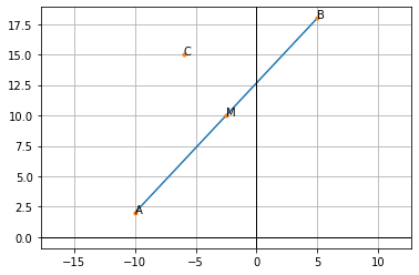
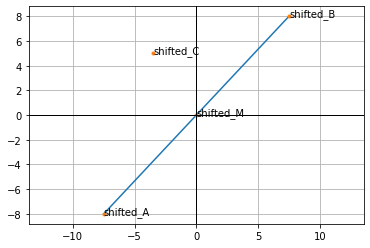
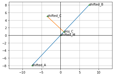
As we can see, the line doesn’t pass through the origin. We have to apply affine transformation to shift the whole space, placing the midpoint AB at (0, 0). If we do so, we can easily find orthogonal projection of the point C on the line ‘marked’ by the B vector. After we shift the space, the segment $MB$ becomes a vector as it has its start in the origin.
transform_matrix = np.eye(3)
transform_matrix[0:2, -1] = -M
transform_matrix
array([[  1. ,   0. ,   2.5],
       [  0. ,   1. , -10. ],
       [  0. ,   0. ,   1. ]])
If you’d like to know more details, how to construct the transformation matrix, see for example Affine Transformation Matrices.
# tranformed_a = affine_transform_matrix @ np.vstack(a.T, [1])
def extend_with_one(vec):
    vec = vec[np.newaxis].T
    return np.vstack([vec, [1]])

transposed  = [extend_with_one(p) for p in points]
transformed = [transform_matrix @ vec for vec in transposed]
# Removing last dimension with '1'
transformed = [vec[0:2] for vec in transformed]
aff_A, aff_B, aff_M, aff_C = transformed

lines  = [[aff_A, aff_B]]
labels = ['shifted_A', 'shifted_B', 'shifted_M', 'shifted_C']

plot(transformed, lines, labels)
Scalar projection
We want to compute the scalar projection of $\bf{v}$ on $\bf{w}$ using the left-hand side of the following equation:
When $\theta$ is the angle between $\bf{w}$ and $\bf{v}$, and $\hat{\bf{w}}$ is the unit vector, namely:
See also:
unit_vec = (aff_B) / np.linalg.norm(aff_B)
scalar_projection = unit_vec.T @ aff_C
scalar_projection
array([[1.25389207]])
# We compute projection of C to draw a plot
proj_C = unit_vec * scalar_projection
# Plot
points = transformed + [proj_C]
lines  = [[aff_A, aff_B], [aff_C, proj_C]]
labels = ['shifted_A', 'shifted_B', 'shifted_M', 'shifted_C', 'proj_C']
plot(points, lines, labels)
Axis class
Rewriting all as a class:
class axis:

    def __init__(self, negative_pole: npt.NDArray, positive_pole: npt.NDArray):

        self.dims = len(negative_pole)

        # Original values
        self.negative_pole = negative_pole
        self.positive_pole = positive_pole
        self.midpoint = _midpoint(negative_pole, positive_pole)

        # Transformation
        self.transform = _transformation_matrix(self.dims, self.midpoint)
        self.shifted_negative_pole = self._shift(negative_pole)
        self.shifted_positive_pole = self._shift(positive_pole)

        self.unit_vector = self.shifted_positive_pole / np.linalg.norm(self.shifted_positive_pole)      # shifted_midpoint is (0, 0, ...)

    def __call__(self, vector: npt.NDArray):

        if (len(vector) != self.dims):
            raise ValueError(
                f'Vector length is {len(vector)}, but it should equal {self.dims}'
            )

        shifted_vector = self._shift(vector)
        return (self.unit_vector.T @ shifted_vector)[0, 0]

    def plot(self, *args, title = "Embedding vectors", figsize = (10, 5),
             poles = {'negative': {'label': 'Negative pole', 'color': 'blue'},
                      'positive': {'label': 'Positive pole', 'color':'red'}}):

        # Init plot
        fig, ax = plt.subplots(figsize=figsize, constrained_layout=True)
        ax.set(title=title)

        # Horizontal line
        neg_value = self(self.negative_pole)
        pos_value = self(self.positive_pole)

        all_values = reduce(add, [a['values'] for a in args])
        all_values = all_values + [neg_value, pos_value]

        ax.plot(all_values, np.zeros_like(all_values), "-o",
        color="k", markerfacecolor="w")  # Baseline and markers on it.

        # Generate colours if not defined
        for group in args:

            values = group['values']
            labels = group['labels']
            color  = group['color']

            levels = np.tile([-5, 5, -3, 3, -1, 1],
                 int(np.ceil(len(values)/6)))[:len(values)]

            ax.vlines(values, 0, levels, color=color)
            vert = np.array(['top', 'bottom'])[(levels > 0).astype(int)]

            for d, l, r, va in zip(values, levels, labels, vert):
                ax.annotate(r, xy=(d, l), xytext=(1, np.sign(l)*3),
                            textcoords="offset points", va=va, ha="right")

        # Show poles
        neg_pole = poles['negative']
        pos_pole = poles['positive']

        ax.vlines(neg_value, 0, 4, neg_pole['color'])
        ax.annotate(neg_pole['label'], xy=(neg_value, 4), xytext=(4, np.sign(4)*3),
            textcoords="offset points", va=va, ha="right", weight='bold')

        ax.vlines(pos_value, 0, 4, color=pos_pole['color'])
        ax.annotate(pos_pole['label'], xy=(pos_value, 4), xytext=(4, np.sign(4)*3),
            textcoords="offset points", va=va, ha="right", weight='bold')

        # Show the plot
        ax.yaxis.set_visible(False)
        ax.spines[["left", "top", "right"]].set_visible(False)
        ax.margins(y=0.1)
        plt.show()

    def _shift(self, vector: npt.NDArray):
        extended_vector = _extend_with_one(vector)
        return (self.transform @ extended_vector)[0:self.dims]


def _extend_with_one(vector: npt.NDArray) -> npt.NDArray:
    vector = vector[np.newaxis].T
    return np.vstack([vector, [1]])

def _transformation_matrix(dims: int, midpoint: npt.NDArray) -> npt.NDArray:
    mat = np.eye(dims + 1)
    mat[0:dims, -1] = -midpoint
    return mat

def _midpoint(x: npt.NDArray, y: npt.NDArray) -> npt.NDArray:
    if (len(x) != len(y)):
        raise ValueError(
            f'Vectors come from different spaces! ' +
            f'x: {len(x)} dimensions, y: {len(y)} dimensions')
    return (x + y) / 2
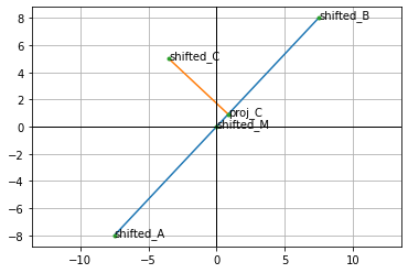
Last quick check with a simplified example:
# Points lying on the straight line
A = np.array([-10, 2])
B = np.array([5, 18]) # 18
C = np.array([-6, 15])

axis_a_b = axis(A, B)

points = [A, B, C, axis_a_b.midpoint]
shifted_points = [axis_a_b._shift(p) for p in points]
proj_C = axis_a_b(C) * axis_a_b.unit_vector
shifted_points = shifted_points + [proj_C]

shifted_A, shifted_B, shifted_C, shifted_M, _  = shifted_points

lines  = [[shifted_A, shifted_B], [shifted_C, proj_C]]
labels = ['shifted_A', 'shifted_B', 'shifted_C', 'shifted_M', 'proj_C']
plot(shifted_points, lines, labels)
Experiment with embeddings
ice_fire_axis = axis(ice.vector, fire.vector)
# Ice
ice_value = ice_fire_axis(ice.vector)

# Fire
fire_value = ice_fire_axis(fire.vector)
cold = ['polar', 'snow', 'winter', 'fridge', 'Antarctica', 'freeze']
warm = ['tropical', 'sun', 'summer', 'oven', 'Africa', 'flame']
cold_vecs = [nlp(w).vector for w in cold]
warm_vecs = [nlp(w).vector for w in warm]
cold_values = [ice_fire_axis(p) for p in cold_vecs]
warm_values = [ice_fire_axis(p) for p in warm_vecs]
warm_values
[-0.179010129140625,
 0.7686063030627324,
 0.21483235444847368,
 0.5769307333087565,
 0.830039105765312,
 2.751032938467553]
all_values = cold_values + warm_values + [ice_value, fire_value]
all_labels = cold + warm
ice_fire_axis.plot(
        {'values': cold_values, 'labels': cold, 'color': 'tab:blue'},
        {'values': warm_values, 'labels': warm, 'color': 'tab:red'},
        poles = {'negative': {'label': 'ice', 'color': 'blue'},
                 'positive': {'label': 'fire', 'color': 'red'}}
    )
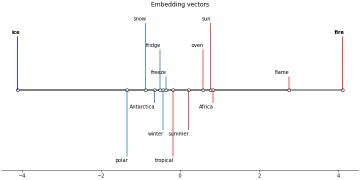
Conclusions
As we can see, in this case the meaning of the mutual position of “ice” and “fire” looks as expected. “Cold words” are closer to the negative pole while the “warm words* - to the positive pole.
To do a similar experiment by yourself, you can use my salto package.