Preparing input for time series models • aion

In this vignette we’ll see, how to prepare an input to the time series deep learning models. To do so quickly, we’ll use functions from {aion} package.

library(data.table)
library(dplyr, warn.conflicts = FALSE)
library(aion)
library(keras)
library(tsibbledata)
library(recipes, warn.conflicts = FALSE)
library(ggplot2)

set.seed(7)

We feed a keras models in two ways, using:

arrays
generators

Below I present, how to prepare both types of inputs/outputs using {aion}.

Data analysis

As an example we’ll the global_economy dataset from the tsibbledata package.

global_economy is a n example of panel dataset. It simply means that in contains multiple time series, distinguished with Country What we’d like to do, after optional preprocessing such as scaling, imputation etc. is to create a set of arrays (tensors) or a generator, which serves respective batch-level tensors on fly.

head(global_economy)
#> # A tibble: 6 × 9
#>   Country     Code   Year         GDP Growth   CPI Imports Exports Population
#>   <fct>       <fct> <dbl>       <dbl>  <dbl> <dbl>   <dbl>   <dbl>      <dbl>
#> 1 Afghanistan AFG    1960  537777811.     NA    NA    7.02    4.13    8996351
#> 2 Afghanistan AFG    1961  548888896.     NA    NA    8.10    4.45    9166764
#> 3 Afghanistan AFG    1962  546666678.     NA    NA    9.35    4.88    9345868
#> 4 Afghanistan AFG    1963  751111191.     NA    NA   16.9     9.17    9533954
#> 5 Afghanistan AFG    1964  800000044.     NA    NA   18.1     8.89    9731361
#> 6 Afghanistan AFG    1965 1006666638.     NA    NA   21.4    11.3     9938414

summary(global_economy$Year)
#>    Min. 1st Qu.  Median    Mean 3rd Qu.    Max. 
#>    1960    1974    1989    1989    2003    2017

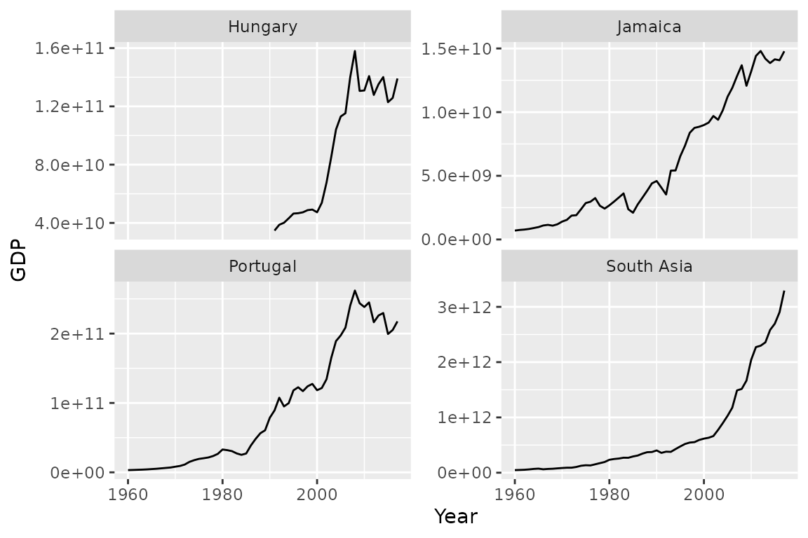
glob_econ <- as.data.table(global_economy)

sample_countries <- sample(unique(global_economy$Country), 4)

ggplot(glob_econ[Country %in% sample_countries]) +
  geom_line(aes(Year, GDP)) +
  facet_wrap(vars(Country), scales = 'free_y')
#> Warning: Removed 31 row(s) containing missing values (geom_path).

Data preprocessing

split_year <- 2000

ge_recipe <- 
  recipe(GDP ~ . , data = glob_econ) %>% 
  step_mutate(Country_idx = Country) %>% 
  step_integer(Country_idx) %>% 
  prep()

train <- 
  glob_econ[Year <= split_year] %>% 
  bake(ge_recipe, .)

test <- 
  glob_econ[Year > split_year] %>% 
  bake(ge_recipe, .)

Arrays

Typically, in the time series forecasting field, we can distiguish the following types of variables:

past values of the target variable
future values of the target variable
past dynamic features (numeric and categorical)
future dynamic features (numeric and categorical)
static features (numeric and categorical)

Past target values can be simply treated as a part of the tensor of the past dynamic features.

The simplest possible scenario is to split the dataset using certain date.

KEY         <- 'Country'
INDEX       <- 'Year'
TARGET      <- 'GDP'
NUMERIC     <- c('Growth', 'CPI', 'Imports', 'Exports', 'Population')
CATEGORICAL <- 'Country_idx'
STATIC      <- 'Country_idx'

LOOKBACK <- 10
HOIRZON  <- 5

train_arrays <-
  make_arrays(
    data        = train,
    key         = KEY,
    index       = INDEX,
    lookback    = LOOKBACK,
    horizon     = HOIRZON,
    stride      = 4,
    shuffle     = TRUE,
    target      = TARGET,
    categorical = CATEGORICAL,
    numeric     = NUMERIC
  )
#> Warning in make_arrays(data = train, key = KEY, index = INDEX, lookback =
#> LOOKBACK, : Found samples with end_time - start_time < total_window_length.
#> They'll be removed.

print(names(train_arrays))
#> [1] "X_past_num" "X_past_cat" "y_fut"      "X_fut_num"  "X_fut_cat"
print(dim(train_arrays$X_past_num))
#> [1] 1820   10    6

As you can see, it contains five types of arrays. One of them, y_fut is the target, while the rest may be used as the model input. To demonstrate, how we can manipulate the data with make_arrays function, let’s add static variables and a separarte array for past GDP values.

train_arrays <-
  make_arrays(
    data        = train,
    key         = KEY,
    index       = INDEX,
    lookback    = LOOKBACK,
    horizon     = HOIRZON,
    stride      = 4,
    shuffle     = TRUE,
    target      = TARGET,
    categorical = CATEGORICAL,
    numeric     = NUMERIC,
    static      = STATIC,
    y_past_sep  = TRUE 
  )
#> Warning in make_arrays(data = train, key = KEY, index = INDEX, lookback =
#> LOOKBACK, : Found samples with end_time - start_time < total_window_length.
#> They'll be removed.

print(names(train_arrays))
#> [1] "y_past"       "X_past_num"   "X_past_cat"   "y_fut"        "X_fut_num"   
#> [6] "X_fut_cat"    "X_static_cat"
print(dim(train_arrays$X_past_num))
#> [1] 1820   10    5

Generators

c(train_gen, train_n_steps) %<-%
  ts_generator(
    data        = train,
    key         = KEY,
    index       = INDEX,
    lookback    = LOOKBACK,
    horizon     = HOIRZON,
    stride      = 4,
    shuffle     = TRUE,
    target      = TARGET,
    categorical = CATEGORICAL,
    numeric     = NUMERIC,
    static      = STATIC,
    y_past_sep  = TRUE,
    batch_size  = 32 
  )
#> Warning in ts_generator(data = train, key = KEY, index = INDEX, lookback =
#> LOOKBACK, : Found samples with end_time - start_time < total_window_length.
#> They'll be removed.

print(class(train_gen))
#> [1] "function"

As we can see, the output is not list of arrays, but a list of two objects:

generator function
Returns a batch of training data at every call. After the loop comes to the end, the counter is reset and the generator starts serving the same data from the beginning again.
number of steps
An argument required by the keras methods.

batch <- train_gen()
names(batch)
#> [1] "y_past"       "X_past_num"   "X_past_cat"   "y_fut"        "X_fut_num"   
#> [6] "X_fut_cat"    "X_static_cat"
print(dim(batch$y_past))
#> [1] 32 10  1

We can them pass these arguments to the fit function as follows:

model %>% 
  fit(
    x = train_gen,
    steps_per_epoch = train_n_steps,
    validation_data = val_gen,
    validation_steps = val_n_steps
  )

model %>% 
  predict(
    x = test_gen,
    steps = test_n_steps
  )